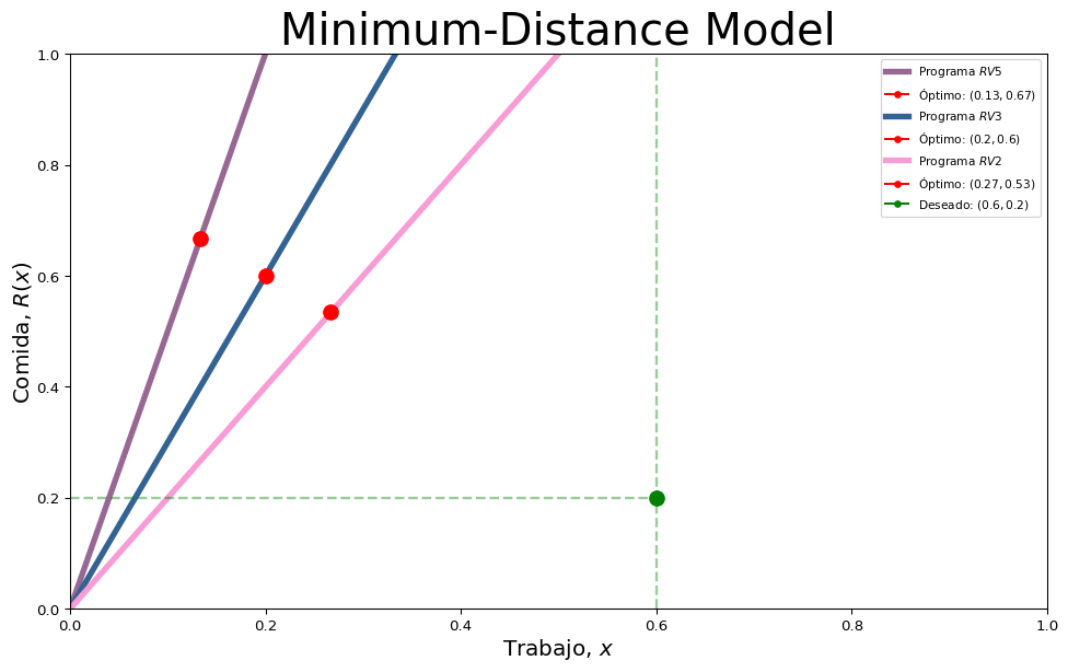
```{python}
# Minimum-Distance Model
import numpy as np
import matplotlib.pyplot as plt


# Bleassing point
R_0, r_0, = 0.6, 0.2

if r_0 + R_0 >= 1:
    y_0  =  0
else:
    y_0 = 1 - r_0 - R_0

rv = [5, 3, 2]
# Linear constants
a, b, c = 0.02, 0.1, 1
# Ratio variable schedule
R = np.linspace(0, 2, 1000)

# Gráfica.
fig, ax = plt.subplots(figsize= (12, 7))

## Límites dinámicos
#if R[-1]/ max(rv) > R_0:
#        ax.set_ylim(0, R[-1]/ rv + 0.5)
#else:
#        ax.set_ylim(0, R_0 + 0.5)

ax.set_ylim(0, 1)
ax.set_xlim(0, 1)

colors = ["#976894", "#336392", "#F79CD4"]
count = 0
for i in rv:
    r_x = R/(i)
    # Sistema de Multiplicadores de Langrage
    #Matriz: R, r, y, l1, l2
    X = np.matrix([[2*a**2, 0, 0, -1, -1],
                [0, 2*b**2, 0, -1, i],
                [0, 0, 2*c**2, -1, 0],
                [-1, -1, -1, 0, 0],
                [-1, i, 0, 0, 0]])

    B = np.matrix([[(2*a**2)*r_0],
                [(2 * b **2)* R_0],
                [(2*c**2)*y_0],
                [-1],
                [0]])

    optimal_points = X.I.dot(B)

    # Reinforcement schedule, Bless Point and optimal point
    ax.plot(r_x, R, color = colors[count], lw = 4, label = f"Programa $RV{rv[count]}$")

    ax.plot(optimal_points[1], optimal_points[0], marker = "o", markersize = 10, color = "red",
            label = f"Óptimo: $({round(float(optimal_points[1]), 2)}, {round(float(optimal_points[0]), 2)} )$")

    count += 1

ax.plot(R_0, r_0, marker = "o", markersize = 10, color = "green",  label = f"Deseado: $({round(R_0, 3)}, {round(r_0, 3)})$")

# The two possible limits
ax.hlines(r_0, 0, R_0, linestyles="dashed", lw = 1.75, alpha = 0.4, color = 'green')
ax.vlines(R_0, 0, 1, linestyles="dashed", lw = 1.75, alpha = 0.4, color = 'green')

# Axis labels
ax.set_title('Minimum-Distance Model', pad=3, fontsize = 30)
ax.set_ylabel(r"Comida, $R(x)$", size = 15, labelpad=2)
ax.set_xlabel(r"Trabajo, $x$", size = 15, labelpad=2)

plt.legend(fontsize = 8, loc = 1, markerscale= 0.4)

plt.show()
```